|
Getting your Trinity Audio player ready... |
When working with data in machine learning, understanding basic statistical concepts is essential. Among these, mean, median, and mode are the most common measures of central tendency — numbers that summarize the center point of your dataset.
These concepts help data scientists understand data distribution, detect anomalies, and preprocess data before feeding it into models.
In this article, we’ll explore:
- What mean, median, and mode are
- How they are calculated
- Their role in machine learning
- Python examples
1. Mean (Average)
The mean is the sum of all values divided by the total number of values.
Formula: Mean=Sum of all valuesNumber of values\text{Mean} = \frac{\text{Sum of all values}}{\text{Number of values}}
Example:
data = [2, 4, 6, 8, 10]
mean = sum(data) / len(data)
print(mean)  # Output: 6.0
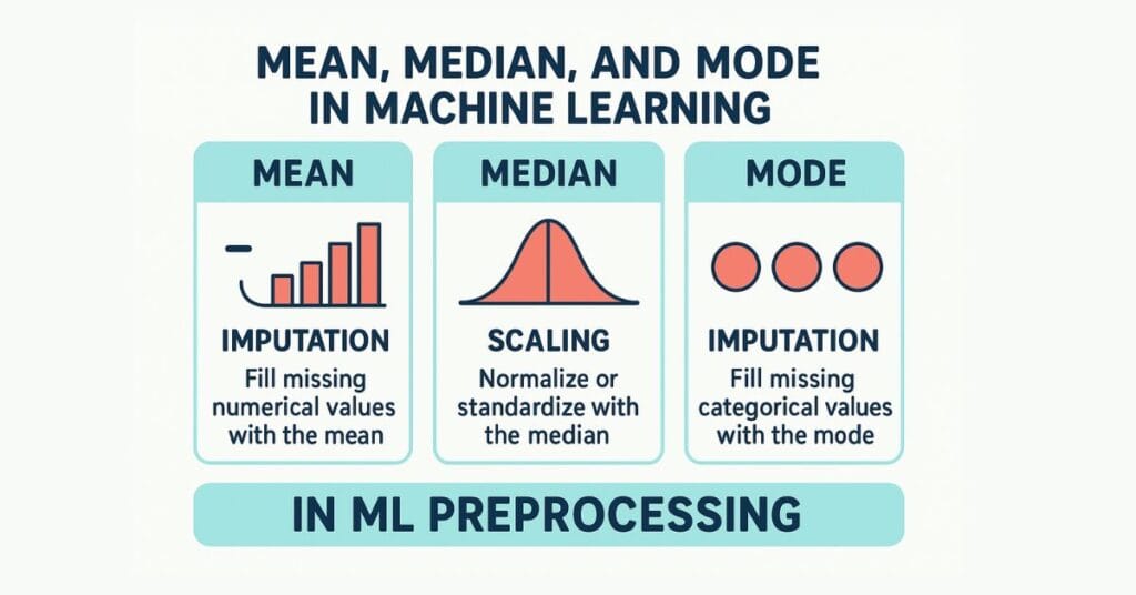
In Machine Learning:
- Used in feature scaling (normalization, standardization)
- Helps understand average trends in data
- Can be misleading if the dataset has outliers (extremely high/low values)
2. Median
The median is the middle value when data is sorted.
- If there’s an odd number of values → middle value is the median.
- If there’s an even number → median is the average of the two middle values.
Example:
import statistics

data = [2, 4, 6, 8, 10]
median = statistics.median(data)
print(median)  # Output: 6
In Machine Learning:
- More robust to outliers compared to mean
- Useful in skewed datasets where mean might be misleading
- Often used in median imputation for missing values
3. Mode
The mode is the most frequently occurring value in a dataset.
Example:
import statistics

data = [2, 4, 4, 6, 8, 10]
mode = statistics.mode(data)
print(mode)  # Output: 4
In Machine Learning:
- Helps identify most common category in classification problems
- Useful in categorical data analysis
- Can be used for mode imputation for missing categorical values
Mean vs Median vs Mode – When to Use
| Measure | Best for | Sensitive to Outliers? |
|---|---|---|
| Mean | Normally distributed data | Yes |
| Median | Skewed data, outlier-prone data | No |
| Mode | Categorical or discrete data | No (but may vary) |
Example: Why This Matters in ML
Imagine you have income data for 10 people (in $1000s):
[30, 35, 28, 40, 32, 31, 120, 34, 33, 29]
- Mean: ~41.2 → Skewed by the $120k outlier
- Median: 33.5 → Better representation of “typical” income
- Mode: 30, 31, 32… (if frequencies tie, there may be multiple modes)
For predictive modeling, using median here would give a better understanding of central value without being misled by the outlier.
Python Quick Summary
import statistics

data = [30, 35, 28, 40, 32, 31, 120, 34, 33, 29]

mean = statistics.mean(data)
median = statistics.median(data)
mode = statistics.multimode(data)  # Returns all modes

print(f"Mean: {mean}")
print(f"Median: {median}")
print(f"Mode: {mode}")
Key Takeaways
- Mean is best for normally distributed data without extreme outliers.
- Median is better when your data is skewed.
- Mode is useful for categorical and discrete values.
- In machine learning, choosing the right measure helps with data preprocessing, feature engineering, and model performance.
4. Real-World Machine Learning Examples
Example 1: Handling Missing Values
Missing data is common in real-world datasets. If not handled properly, it can reduce model accuracy or even cause errors during training.
Dataset Example:
import pandas as pd
import numpy as np

df = pd.DataFrame({
    'Age': [25, 30, np.nan, 40, 35, np.nan, 50],
    'Salary': [40000, 50000, 60000, np.nan, 45000, 52000, 58000],
    'Department': ['IT', 'HR', 'IT', 'Finance', 'Finance', np.nan, 'HR']
})
print(df)
Filling Missing Values:
- Mean imputation (good for normally distributed numeric data):
df['Salary'].fillna(df['Salary'].mean(), inplace=True)
- Median imputation (better for skewed data):
df['Age'].fillna(df['Age'].median(), inplace=True)
- Mode imputation (for categorical data):
df['Department'].fillna(df['Department'].mode()[0], inplace=True)
Example 2: Outlier Impact on Model Accuracy
Let’s see how mean vs median affects preprocessing.
Problem:
A dataset has an extreme salary value:
salaries = [40000, 42000, 41000, 39000, 1000000] # Outlier present
- Mean salary = 216,000 → Unrealistic average for most people in the dataset
- Median salary = 41,000 → Represents typical value
If you use the mean for scaling, your model might think salaries are much higher than they really are, which could distort regression predictions.
Example 3: Predicting Housing Prices
In housing datasets:
- Mean price can be skewed by luxury mansions
- Median price better reflects what an “average” home costs
- Mode is useful for most common house features (like number of bedrooms)
import statistics

prices = [150000, 160000, 155000, 2000000, 158000]
print("Mean Price:", statistics.mean(prices))
print("Median Price:", statistics.median(prices))
In machine learning models (like Linear Regression), using the median as a target transformation can make the model more robust to extreme values.
Conclusion
In machine learning:
- Mean is quick but sensitive to outliers
- Median is safer for skewed data
- Mode is essential for categorical variables
When cleaning and preprocessing data, choosing the right measure can improve model accuracy and reduce bias.
🔗 Originally published on Makemychance.com

Arsalan Malik is a passionate Software Engineer and the Founder of Makemychance.com. A proud CDAC-qualified developer, Arsalan specializes in full-stack web development, with expertise in technologies like Node.js, PHP, WordPress, React, and modern CSS frameworks.
He actively shares his knowledge and insights with the developer community on platforms like Dev.to and engages with professionals worldwide through LinkedIn.
Arsalan believes in building real-world projects that not only solve problems but also educate and empower users. His mission is to make technology simple, accessible, and impactful for everyone.
Join us on dev community